From RLHF to Direct Preference Learning

It’s well known that the state-of-the-art LLM models are trained with massive human quality feedback. This feedback is either coming from a massive rater pool, or can come from the end users implicitly (sometimes explicitly as well.. remember when ChatGPT presents you 2 responses to choose from?).

However, I found that there are many subtleties for one to truly understand what’s going on under the hood. This is a blog to capture my understanding of the RLHF algorithm, and how it evolves into rewardless model such as DPO and IPO.

A quick recap of RLHF

Suppose our reward is point-wise, meaning we get a single float number to denote the quality of the response based on the context, we try to optimize for the following objective in RLHF

$$ \begin{equation} \begin{aligned} J(\pi) &= \mathbb{E}_{\substack{x \sim D \\ y \sim \pi(\cdot|x)}} \left[ r(x, y) \right] - \beta\mathbb{D}_\text{KL}(\pi ||\pi_\text{ref}) \end{aligned} \end{equation} $$

The reward function \( r(x, y) \) usually isn't directly differentiable in relative to \(\pi\) itself (for example, in auto-regressive model where we sample each token with argmax). Thus the most common approach to deal with this case is to use actor critic method to find the best policy.

Optimizing equation (1) usually consists of the following general steps, assuming we are using PPO

1. Training the reward model

Suppose we have access of many \( (\text{prompt}, \text{likert score}) \) pairs, we can train the reward model \( r(x, y) \) with MSE loss and with a neural network. One good thing is that such neural network can be directly initialized with the underlying policy transformer network, and replace the output layers to be a shallow FFN.

2. Sample the policy, and estimate value

During this step, suppose we have access to many prompts that matches the distribution we want to optimize, say \( x \sim D \), we can thus run the policy \(T\) times and send the responses for reward scoring. This will results a distribution \( \text{M} \) with \(T\) episodes where each episode \( \text{M}^t \) consists of:

$$ \text{M}^t = (\text{prompt x}^t, \text{response y}^t, \text{score r}^t, \text{value v}^t, \text{probability p}^t) $$

Additionally, we also generate 2 more things:

• value: This is generated by a value network, which is needed to stabilize the RL training to make it offset invariant. See PPO paper for details. One good thing about it is that such value network can be initialized by the policy SFT’ed network too, similar to our reward model.
• probability: This is the probability of the response sequence (of length n), equals to $$ \prod_{i=1}^{n} p(y_i \mid y_1, y_2, \ldots, y_{i-1}, x) $$ this will later be used to calculate the KL divergence.

3. Train with PPO

Following the common PPO training, we have the loss function across all the \(T\) episodes as

$$ \begin{aligned} L^{\text{PPO}}(\pi) = \mathbb{E}_{t \sim M} \Bigg[ & \min \left( \rho_t(\pi) \hat{A}_t, \text{clip} \left( \rho_t(\pi), 1 - \epsilon, 1 + \epsilon \right) \hat{A}_t \right) \Bigg] \end{aligned} $$

where, $$ \begin{aligned} \rho_t(\pi) &= \frac{\pi(y^t | x^t)}{\pi_{\text{ref}}(y^t | x^t)} \\ \hat{A}_t &= J_t - v^t \\ J_t &= r^t - \beta\mathbb{D}_{\text{KL}}(\pi || \pi_{\text{ref}}) \end{aligned} $$

I think it’s worth pointing out the calculation of the KL divergence (at least it took me a long time to figure out). The definition of KL divergence is

$$ D_{\text{KL}}(\pi \parallel \pi_{\text{ref}}) = \sum_{y} \pi(y|x) \log \left( \frac{\pi(y|x)}{\pi_{\text{ref}}(y|x)} \right) $$

comprehensively evaluate for all y is computationally intractable (like, you need to exhaust all possible human sentences). But recall that the meaning of KL divergence is measure how different 2 distribution is, and that can also be translated to how different 2 distribution assign probability to the same sequence sample from one of them¹.

Thus a noisy estimation of the KL divergence can be expressed as

$$ D_{\text{KL}}(\pi \parallel \pi_{\text{ref}}) = \mathbb{E}_{x \sim M}[\text{KL}(\pi(\cdot|x) || \pi_{\text{ref}}(\cdot|x))] $$

where

$$ \mathbb{E}_{x \sim M}[\text{KL}(\pi(\cdot|x) || \pi_{\text{ref}}(\cdot|x))] = \mathbb{E}_{y \sim \pi(\cdot|x)}\Bigg[\log(\frac{\pi(y|x)}{\pi_{\text{ref}(y|x)}}) \Bigg] $$

You can also check this implementation to gain a deeper understanding of it.

4. Update value estimator

Finally, once the model has been updated, the value function is fitting to the actual reward. You repeat 2-4 until the model is aligned with the preference.

Deal with pairwise preference

The previous section is assuming a point wise preference labeling, that is, each reward labeling is of pair $$ (\text{prompt}, \text{likert score}) $$ However, human is not very good at rating absolutely, but very good as comparing things side by side. For example, it’s hard to say how hot the weather is exactly in terms of Celsius, but it’s quite easy to tell the the weather in the evening is more chill compared to the afternoon. The same intuition applies for LLM training, while it’s hard to collect absolute likert score, it’s relatively easy to collect a triplet of $$ (\text{prompt}, \text{response}_w, \text{response}_l) $$

Where the 2 responses are 2 samples and we collect the preference score from a rater pool about which one is better (\(\text{response}_w\)) and which one is worse (\(\text{response}_l\)) in the context of the prompt.

Rather than training the reward model to fit the absolute score, the reward model instead trained to fit a Bradley-Terry model ².

Let the prompt be \(x\) and \( \text{response}_w, \text{response}_l \) be \(y_w, y_l\) respectively. The objective instead becomes

$$ L(r) = -\mathbb{E}_{(x, y_w, y_l)}[\log(p(y_w>y_l|x))] $$ where $$ p(y_w>y_l|x) = \sigma(r(x,y_w) - r(x, y_l)) $$

See this implementation to get a deeper understanding of the pairwise reward model training. Once the reward model is trained, we use PPO with the same objective as in equation (1) to perform RLHF.

DPO: Avoid the reinforcement learning at all

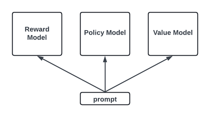
Let’s recap, in RLHF (with PPO), we need to bring up 3 models to do different things. We need our policy model to create episodes and update, a reward model to score the generated response and a value model to estimate the value in order to stabilize the training. Although theoretically a lot of parameters can be shared across them ³, it is still relatively resource intensive compared to instruction fine tuning. In addition, it requires an additional step to train the reward model, which leaves more room for error.

Thus, we are interested in a reward free method which can be more resource/time efficient method that can avoid the above issue. And guess what, DPO does exact that with a quite beautiful mathematic trick.

Recall that our objective, even though non differentiable, is $$ \begin{aligned} J(\pi) &= \mathbb{E}_{\substack{x \sim D \\ y \sim \pi(\cdot|x)}} \left[ r(x, y) \right] - \beta\mathbb{D}_\text{KL}(\pi ||\pi_\text{ref}) \end{aligned} $$ Let’s see if we can have an analytic solution to the optimal policy $$ \begin{aligned} \max_\pi J &= \max_\pi\mathbb{E}_{\substack{x \sim D \\ y \sim \pi(\cdot|x)}} \left[ r(x, y) \right] - \beta\mathbb{D}_\text{KL}(\pi ||\pi_\text{ref}) \\ &= \max_\pi\mathbb{E}_{\substack{x \sim D \\ y \sim \pi(\cdot|x)}} \left[ r(x, y) \right] - \beta\mathbb{E}_{\substack{x \sim D \\ y \sim \pi(\cdot|x)}}\Bigg[\log(\frac{\pi(y|x)}{\pi_{\text{ref}}(y|x)})\Bigg] \\ &= \max_\pi\mathbb{E}_{\substack{x \sim D \\ y \sim \pi(\cdot|x)}} \Bigg[ r(x, y) - \beta\log(\frac{\pi(y|x)}{\pi_{\text{ref}}(y|x)})\Bigg] \\ &= \min_\pi\mathbb{E}_{\substack{x \sim D \\ y \sim \pi(\cdot|x)}} \Bigg[ \beta\log(\frac{\pi(y|x)}{\pi_{\text{ref}}(y|x)}) - r(x, y) \Bigg] \\ &= \min_\pi\mathbb{E}_{\substack{x \sim D \\ y \sim \pi(\cdot|x)}} \Bigg[ \beta\log(\frac{\pi(y|x)}{\pi_{\text{ref}}(y|x)\cdot\exp(\frac{1}{\beta}r(x, y))}) \Bigg] \\ &= \beta\min_\pi\mathbb{E}_{\substack{x \sim D \\ y \sim \pi(\cdot|x)}} \Bigg[ \log{\frac{\pi(y|x)}{\frac{1}{Z(x)}\pi_{\text{ref}}(y|x)\cdot\exp(\frac{1}{\beta}r(x, y))}} - \log{Z(x)}\Bigg] \\ \end{aligned} $$

let \(Z(x) = \sum_{\text{all of } y \sim \pi(\cdot|x)}{\pi_{\text{ref}}(y|x)\exp(\frac{1}{\beta}r(x, y))} \), we can see that the denominator in the above equation is a valid distribution (probability adds up to 1). Thus, the objective function becomes

$$ \begin{equation} \begin{aligned} \max_\pi J &= \beta\min_\pi\mathbb{E}_{x \sim D } [\mathbb{D}_\text{KL}(\pi(y|x) ||\pi_*(y|x)) - \log{Z(x)}] \end{aligned} \end{equation} $$ where $$ \begin{equation} \pi_*(y|x) = \frac{1}{Z(x)}\pi_{\text{ref}}(y|x)\cdot\exp(\frac{1}{\beta}r(x, y)) \end{equation} $$

because \(Z(x)\) is exactly irrelevant to \(\pi\), we know that solution to equation (2) is \(\pi = \pi_*\). Thus equation (3) is our optimal policy model that perfectly aligns with the reward model.

Up until know, our conclusion in (3) doesn't help so much. That's because we have a nasty term \(Z(x)\) which requires up to calculate the probability of all possible y given x which is impractical in practice.

But here comes the fun part: With some mathematic tricks, we can cancel out the incomputable Z and get a computable loss function!:

To see how, let's assume our reward model \(r^*\) fits the human preference with a Bradley-Terry model. That is, we have

$$ \begin{equation} p(y_w>y_l|x) = \sigma(r(x, y_w) - r(x, y_l)) \end{equation} $$

Because we have \(\pi_*(y|x) = \frac{1}{Z(x)}\pi_{\text{ref}}(y|x)\cdot\exp(\frac{1}{\beta}r(x, y))\), we can reparametrize the optimal reward as

$$ \begin{equation} r(x, y) = \beta\log{\frac{\pi^*(y|x)}{\pi_{\text{ref}}(y|x)}} + \beta\log{Z(x)} \end{equation} $$

If we substitute (5) into (4), surprisingly we canceled out the term Z! And the Bradley-Terry model can be expressed as $$ \begin{equation} p(y_w>y_l|x) = \sigma\Bigg(\beta\log{\frac{\pi^*(y_w|x)}{\pi_{\text{ref}}(y_w|x)}} - \beta\log{\frac{\pi^{\ast}(y_l|x)}{\pi_{\text{ref}}(y_l|x)}}\Bigg) \end{equation} $$

I just want to stop here and appreciate the beauty of the above derivation. Let’s think about what this final equation (6) actually implies:

• Finding the perfect reward model that fits the pair wise preference in (4) is mathematically equivalent to finding a perfect policy model that fits the same pair wise preference.
• Any reward model has a corresponding policy model that captures the same learned preference (equation (3))

Thus, our final objective becomes $$ \begin{equation} L_{\text{DPO}}(\pi;\pi_{\text{ref}})=-\mathbb{E}_{(x,y_w,y_l) \sim D}\Bigg[ \log{\sigma\Bigg(\beta\log{\frac{\pi^*(y_w|x)}{\pi_{\text{ref}}(y_w|x)}} - \beta\log{\frac{\pi^{\ast}(y_l|x)}{\pi_{\text{ref}}(y_l|x)}}\Bigg)} \Bigg] \end{equation} $$

Note that the above objective (7) is differentiable, and thus we don’t need reinforcement learning to learn the objective, but instead can just train the policy model with back propagation! This thus greatly simplifies our training process.

We suggest you to also look at the original DPO paper where it analyze the property of its gradient to build more intuition. But to sum up, the policy model together with the original reference model (SFT model) encodes implicitly the preference in the reward model training dataset. Such preference doesn’t require training a RM as a proxy but instead can directly train the policy model to learn. Due to such simplicity, in fact most of the open source large language model use some version of DPO to train the model.

Limitation of DPO

But is DPO the perfect method to train LLM? Why we never heard that OpenAI is using DPO to perform GPT post-training?

Many works⁴⁵⁶ analyze the problem, and shows that DPO has the following theoretical limitations:

DPO will assign high value to out-of-distribution samples ⁴

Suppose we have only 3 actions listed in the table below

Action	y1	y2	y3
πref	0.5	0.5	0
Dpref	{(yw = y1, yl = y2)}
πDPO	0.1	0.0	0.9
πPPO	1	0	0

We can see that DPO can learn the solution of 0.1, 0, 0.9. This is because the reward function

$$ \begin{aligned} L_{\text{DPO}}(\pi;\pi_{\text{ref}})& =-\mathbb{E}_{(x,y_w,y_l) \sim D}\Bigg[ \log{\sigma\Bigg(\beta\log{\frac{\pi^*(y_w|x)}{\pi_{\text{ref}}(y_w|x)}} - \beta\log{\frac{\pi^{\ast}(y_l|x)}{\pi_{\text{ref}}(y_l|x)}}\Bigg)} \Bigg] \\ &= -\log{\sigma\Bigg(\beta(\log(\frac{a}{0.5})-\log{\frac{b}{0.5}})\Bigg)} \\ &= \log\Bigg(1+(\frac{a}{b})^\beta\Bigg) \end{aligned} $$

Thus as long as \(a=0\), it is an optimal policy from the view of DPO. However, such policy won't be an optimal one for PPO training, as the KL divergence will ensure the model to stay close to the reference model.

This is also discovered in the Nvidia Nemotron⁵ training, where in the tech report, they reported that

While the policy learns to differentiate chosen and rejected responses, we observe both chosen and rejected responses’ likelihoods drop consistently with their gap increasing, even if chosen responses are high-quality.

In addition, RLHF with PPO can leverage prompt only date, and such dataset act as a good regularizer of the model training to avoid it bias toward OOD samples.

DPO will overfit when the preference is too deterministic

In DeepMind's analysis, under the assumption that \(p^\ast\) fits a Bradley-Terry model, we can prove that for the learning objective below

$$ \max_\pi\mathbb{E}_{\substack{x \sim D \\ y \sim \pi(\cdot|x) \\ y’ \sim \mu(\cdot|x)}}[\Psi(p^\ast(y>y’|x))] - \tau\mathbb{D}_{\text{KL}}(\pi || \pi_{\text{ref}}) $$

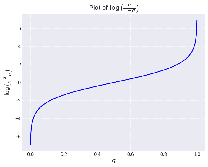
it is exactly the same as the RLHF objective in (1), and thus equivalent to the DPO learning objective in (7), when $$ \Psi(q) = \log(\frac{q}{1-q}) $$

It's actually quite easy to prove this proposition and we leave that to the reader. But looking at the shape of this function, we can see that this function has a very large gradient near the point of 0 and 1. When training with this objective, a small increase in the preference near 0 or 1 will just be as incentivized as a large increase near 0.5. Thus, when the ground truth label is very deterministic (such as machine based feedback), thus no matter how large the regularization term \(\tau\) is, the model will eventually deviate away from the reference and thus overfit drastically.

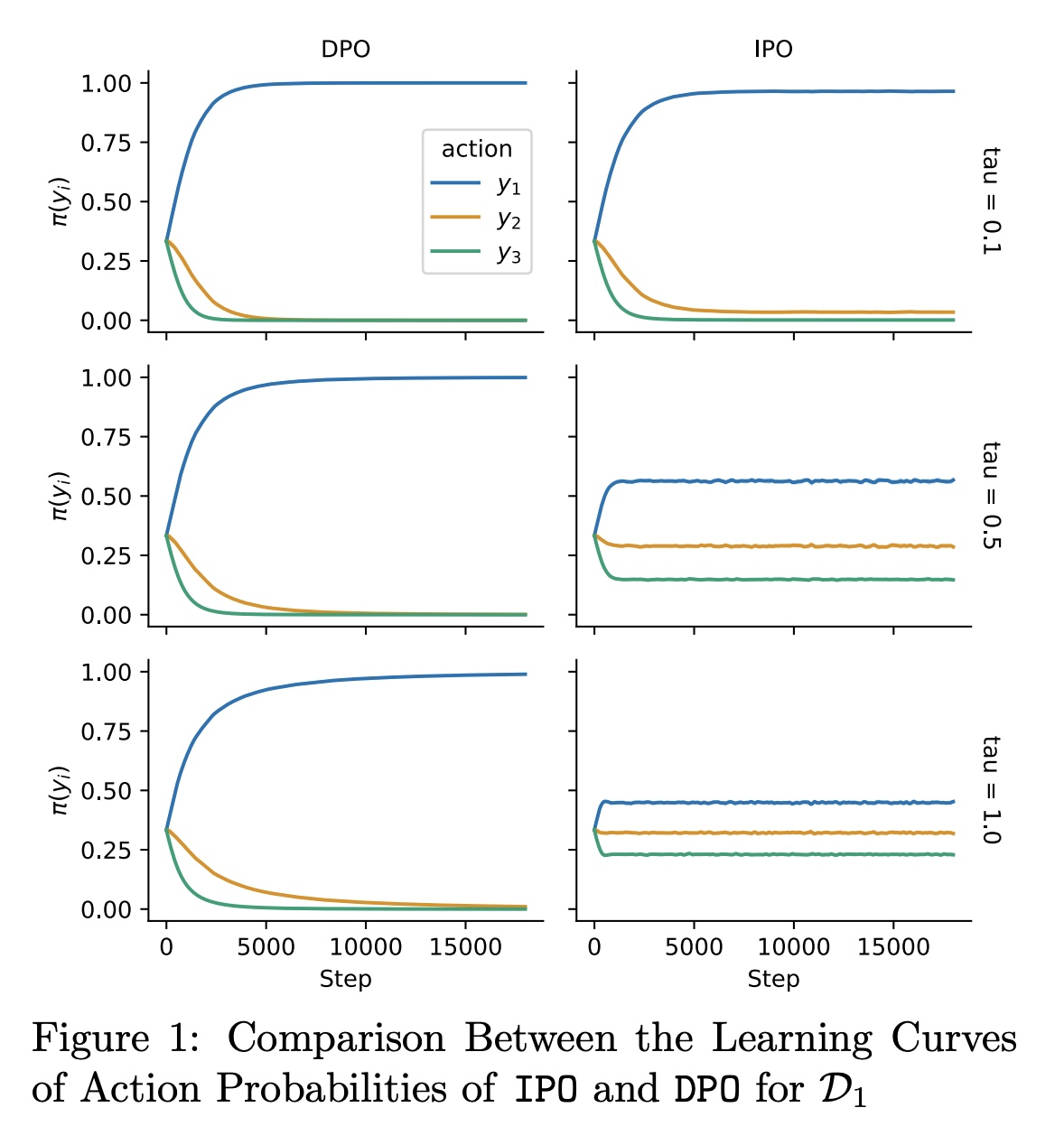
This is also demonstrated in the experiment of IPO, where no matter how large the regularizer is, the policy will eventually deviate away from the original one. However, this won’t happen in RLHF not only because a RM is trained to proxy the raw preference and serves as a regularizer, it utilize PPO which only moves the policy in a trust region. This might be why DeepSeek V2 Coder is using an RM to regularize the execution feedback instead of sending it directly for learning.

Summary

Okay, you made it to the end, congrats :) Before you go, let’s just recap what we have learned:

• RLHF with PPO is the standard way of aligning the post SFT model towards annotated human preference. Pairwise preference is fitted with a Bradley-Terry model.
• DPO utilize a reparametrization trick, and prove that theoretically the policy model captures the preference and can be directly learned via back propagation.
• While DPO is simpler and more computational efficient, it suffers from regularization problem for both OOD and deterministic feedback (such as 0/1), thus while it generally performs well in more subjective tasks where a multi-scale likert score is used, it should be used with caution when the feedback is too deterministic or preference dataset is too small.

I hope you like this post and please don’t hesitate to give your suggestion (scroll all the way up and click “Suggest Changes”). Thanks!